

PyTorch Tutorial 06 - Save and Load the Model
Save and Load the Model — PyTorch Tutorials 2.10.0+cu128 documentation
官方pytorch-tutorial:Learn the Basics 完结篇,本文是 PyTorch 官方 Tutorial 中 Save and Load the Model 部分的学习记录和一些个人补充知识
完结撒花! 这是官方Learn the Basic的最后一篇,因为官方这里讲的内容比较少,个人加了一些相关的补充内容。
Save and Load the Model
官方这里主要是讲了两种保存方式,一种是推荐做法(保存加载权重字典)一种是遗留做法(保存加载整个模型对象)。
Saving and Loading Model Weights
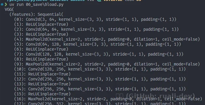
这里以加载来自 models.vgg16()的VGG16网络架构和互联网上的预训练权重为例。
下载:
import torch
import torchvision.models as models

model = models.vgg16(weights='IMAGENET1K_V1')
torch.save(model.state_dict(), 'model_weights.pth')

加载
model = models.vgg16() # we do not specify ``weights``, i.e. create untrained model
model.load_state_dict(torch.load('model_weights.pth', weights_only=True))
model.eval()

print(model) # 打印模型结构
be sure to call model.eval() method before inferencing to set the dropout and batch normalization layers to evaluation mode. Failing to do this will yield inconsistent inference results.
小细节:请务必在推理前调用 model.eval() 方法,将 dropout 和批归一化层设置为评估模式。否则将导致推理结果不一致。(见上篇文章)
Saving and Loading Models with Shapes
这里官方讲的比较简洁:
保存:
When loading model weights, we needed to instantiate the model class first, because the class defines the structure of a network. We might want to save the structure of this class together with the model, in which case we can pass
model(and notmodel.state_dict()) to the saving function:
加载模型权重时,我们需要先实例化模型类,因为该类定义了网络的结构。有时我们希望将此类的结构与模型一同保存,在这种情况下,我们可以将 model(而非 model.state_dict())传递给保存函数:
torch.save(model, 'model.pth')
加载:
model = torch.load('model.pth', weights_only=False)
This approach uses Python pickle module when serializing the model, thus it relies on the actual class definition to be available when loading the model.
此方法在序列化模型时使用 Python pickle 模块,因此它依赖于加载模型时可用的实际类定义。为什么说这个是遗留用法?
因为涉及 pickle 反序列化,有安全与兼容性风险(防止加点恶意代码进去,和奇奇怪怪的路径版本问题)
个人补充
这里官方到上面就结束了,个人补充点东西吧。
首先贴个上一章训练MLP的保存模型的代码。这里设置了保留best.pth和last.pth方便回滚模型:
import torch
from torch import nn
from torch.utils.data import DataLoader
from torchvision import datasets
from torchvision.transforms import ToTensor
from pathlib import Path

training_data = datasets.FashionMNIST(
    root= "data",
    train=True,
    download=True,
    transform=ToTensor()
)

test_data = datasets.FashionMNIST(
    root="data",
    train=False,
    download=True,
    transform=ToTensor()
)

train_dataloader = DataLoader(training_data , batch_size=64)
test_dataloader = DataLoader(test_data , batch_size=64)

class NeuralNetwork(nn.Module):
    def __init__(self):
        super().__init__()
        self.flatten = nn.Flatten()
        self.linear_relu_stack = nn.Sequential(
            nn.Linear(28*28 , 512),
            nn.ReLU(),
            nn.Linear(512,512),
            nn.ReLU(),
            nn.Linear(512,10),
        )

    def forward(self , x):
        x = self.flatten(x)
        logits = self.linear_relu_stack(x)
        return logits

device = "cuda" if torch.cuda.is_available() else "cpu"
model = NeuralNetwork()
model.to(device)
# model.load_state_dict(torch.load('model.pth', weights_only=True))

def train_loop(dataloader , model, loss_fn , optimizer):
    size = len(dataloader.dataset)
    model.train() # 开dropout和BatchNorm


    for batch , (X ,y) in enumerate(dataloader):

        X, y = X.to(device), y.to(device)

        pred = model(X) # 此轮预测输出
        loss = loss_fn(pred , y) # 求误差

        loss.backward() # 反向传播算梯度
        optimizer.step() # 更新模型参数
        optimizer.zero_grad() #清空梯度

        if batch % 100 == 0:
            loss , current = loss.item() , batch * batch_size + len(X)
            print(f"loss: {loss:>7f} [{current:>5d}/{size:>5d}]")

def test_loop(dataloader, model, loss_fn):
    # Set the model to evaluation mode - important for batch normalization and dropout layers
    # Unnecessary in this situation but added for best practices
    model.eval()

    size = len(dataloader.dataset)
    num_batches = len(dataloader)
    test_loss, correct = 0, 0

    # Evaluating the model with torch.no_grad() ensures that no gradients are computed during test mode
    # also serves to reduce unnecessary gradient computations and memory usage for tensors with requires_grad=True
    with torch.no_grad():
        for X, y in dataloader:
            X, y = X.to(device), y.to(device)
            pred = model(X)
            test_loss += loss_fn(pred, y).item()
            correct += (pred.argmax(1) == y).type(torch.float).sum().item() # 这个 batch 里预测对了多少个。

    test_loss /= num_batches # Avg loss = 所有 batch 的 loss 平均
    correct /= size
    print(f"Test Error: \n Accuracy: {(100*correct):>0.1f}%, Avg loss: {test_loss:>8f} \n")
    return test_loss, correct

best_loss = float("inf")

def save_ckpt(model, optimizer, epoch, test_loss, best_loss):
    # 每轮都存 latest(可续训/回滚到最近一次)
    torch.save({
        "epoch": epoch,
        "model": model.state_dict(),
        "optim": optimizer.state_dict(),
        "best_loss": best_loss,
    }, "last.pth")

    # 更好就覆盖 best(回滚用)
    if test_loss < best_loss:
        torch.save({
            "epoch": epoch,
            "model": model.state_dict(),
            "optim": optimizer.state_dict(),
            "best_loss": test_loss,
        }, "best.pth")
        return test_loss, True

    return best_loss, False


# 定义超参
learning_rate = 1e-3
batch_size = 64
epochs = 5

# Optimization Loop

# Initialize the loss function
loss_fn = nn.CrossEntropyLoss() # 直接吃 logits(没 softmax 的原始输出)+ 类别标签 y(整型类标)。


# 优化:在每个训练步骤中调整模型参数以减少模型误差的过程。
# 优化器定义了如何执行此过程
optimizer = torch.optim.SGD(model.parameters(), lr=learning_rate) # SGD 随机梯度下降 Stochastic Gradient Descent

resume_path = Path("last.pth")   # 想从最佳回滚就改成 Path("best.pth")
start_epoch = 0
best_loss = float("inf")

if resume_path.exists():
    ckpt = torch.load(resume_path, weights_only=True, map_location=device)
    model.load_state_dict(ckpt["model"])
    optimizer.load_state_dict(ckpt["optim"])
    start_epoch = ckpt["epoch"] + 1
    best_loss = ckpt.get("best_loss", best_loss)
    print(f"[RESUME] loaded {resume_path} -> start_epoch={start_epoch}, best_loss={best_loss:.6f}")
else:
    print(f"[RESUME] no checkpoint at {resume_path}, train from scratch")


for t in range(start_epoch, start_epoch + epochs): # 总共训练到某个 epoch 数
    """
    epoch(轮次)能继承:你保存了 epoch,
    加载后 start_epoch = ckpt["epoch"] + 1,
    训练循环从那一轮继续。
    """
    print(f"Epoch {t+1}\n-------------------------------")
    train_loop(train_dataloader, model, loss_fn, optimizer)
    test_loss, test_acc = test_loop(test_dataloader, model, loss_fn)
    best_loss, is_best = save_ckpt(model, optimizer, t, test_loss, best_loss)
print("Done!")
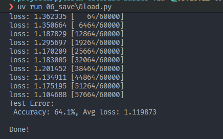
每次训练5轮:
训练了25轮,差不多可以了:
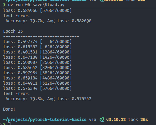
- 3层mlp差不多就到这里了,继续训练收益很小(模型受限于展平输入,缺乏空间归纳偏置),要想效果更好那就改下架构或者优化器啥的,但是这里的话,先讲讲些补充知识。
为什么分Saving and Loading Model Weights/Saving and Loading Models with Shapes:
按照官方这么训练,现在出来的模型是.pth格式。本质就是“纯参数(+少量训练状态)”,它自己并不等于“一个能直接跑的模型”。它必须配合同样的模型结构才能用。
比如说就这个pth,假设我现在要加载推理,我需要先把网络结构搭出来,再把参数按名字对上去:
model = NeuralNetwork()          # 这一步就是“搭网络结构”
state = torch.load("weights.pth", weights_only=True)
model.load_state_dict(state)     # 这一步是“装参数”
为什么说“把参数按名字对上去”?
原因很简单: .pth 里存的 key 是类似这种:
- linear_relu_stack.0.weight
- linear_relu_stack.0.bias
- linear_relu_stack.2.weight
这些 key 只有在你创建了同名层之后,才能“塞进去”。
没有结构,只有一堆张量名字和数值,它自己跑不了。
然而,我们刚刚直接保存模型,受限于底层的pickle,有可能往模型里面塞些恶意代码还有其它奇奇怪怪的问题(见上文),所以说pytorch推荐只保存/加载state_dict。
- 那推理怎么办?
可以导onnx或者其它格式,那就是后话了,此处不赘述。
推理和验证模型效果
这里先不展开部署格式(ONNX/TorchScript),但是刚刚模型都训练了,来把“训练 → 保存 → 加载 → 推理/评估”这条链路跑通:
-
评估(evaluation):有标签,计算
loss/accuracy,用来验证模型整体效果; -
推理(inference):通常没标签,只输出预测类别和置信度。
下面我用 FashionMNIST 的 test 集做一次评估,再随机抽一张图做“单张推理 + 可视化”,把本章闭环补全。
import torch
from torch import nn
from torch.utils.data import DataLoader
from torchvision import datasets
from torchvision.transforms import ToTensor

test_data = datasets.FashionMNIST(
    root="data",
    train=False,
    download=True,
    transform=ToTensor()
)

test_dataloader = DataLoader(test_data , batch_size=64)

class NeuralNetwork(nn.Module):
    def __init__(self):
        super().__init__()
        self.flatten = nn.Flatten()
        self.linear_relu_stack = nn.Sequential(
            nn.Linear(28*28 , 512),
            nn.ReLU(),
            nn.Linear(512,512),
            nn.ReLU(),
            nn.Linear(512,10),
        )

    def forward(self , x):
        x = self.flatten(x)
        logits = self.linear_relu_stack(x)
        return logits

device = "cuda" if torch.cuda.is_available() else "cpu"
model = NeuralNetwork()
ckpt = torch.load("best.pth", weights_only=True, map_location=device)
model.load_state_dict(ckpt["model"])
model.to(device)
model.eval()

# 从 test_data 随机取一张图做推理(带置信度)
# FashionMNIST 的类别名
classes = [
    "T-shirt/top", "Trouser", "Pullover", "Dress", "Coat",
    "Sandal", "Shirt", "Sneaker", "Bag", "Ankle boot"
]

def predict_one(model, img, device, *, topk=1):
    """
    img: torch.Tensor, shape [1,28,28] (FashionMNIST ToTensor 输出)
    return: (pred_idx, conf, probs) 或 topk 列表
    """
    model.eval()

    x = img.unsqueeze(0).to(device)   # [1,1,28,28]
    with torch.inference_mode():
        logits = model(x)             # [1,10]
        probs = torch.softmax(logits, dim=1)[0]  # [10]

    if topk == 1:
        pred = int(probs.argmax().item())
        conf = float(probs[pred].item())
        return pred, conf, probs.cpu()
    else:
        vals, idxs = torch.topk(probs, k=topk)
        out = [(int(i.item()), float(v.item())) for v, i in zip(vals, idxs)]
        return out, probs.cpu()

idx = torch.randint(0, len(test_data), (1,)).item()
img, label = test_data[idx]

pred, conf, probs = predict_one(model, img, device)

print(f"[ONE] idx={idx}")
print(f"  pred: {pred} ({classes[pred]}) conf={conf:.3f}")
print(f"  true: {label} ({classes[label]})")

# 看图
import matplotlib.pyplot as plt

def show_pred(img, pred, conf, label=None):
    plt.imshow(img.squeeze(0), cmap="gray")
    title = f"pred={classes[pred]} ({conf:.2f})"
    if label is not None:
        title += f" | true={classes[label]}"
    plt.title(title)
    plt.axis("off")
    plt.show()

show_pred(img, pred, conf, label)
效果:(传入单张 img(FashionMNIST 取出来那种 [1,28,28] Tensor,出图出预测结果):
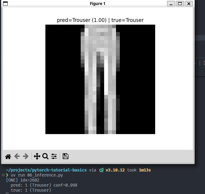
抽到的这个图是Trouser,在 FashionMNIST 里:Trouser的特征就是这样“两条腿”,还是挺好认的。这里置信度0.998。但是,在MLP看来,它“看到的”是“整体像素分布”。学的是像素模式。
另外,这里用的是 Python + PyTorch 做推理验证;真正部署时通常会把训练产物导出成更“推理友好”的格式(比如 ONNX/TorchScript),让推理端不再依赖训练脚本的上下文。本章先不展开部署细节。
结语
到这里,官方 Learn the Basics 就告一段落了。回顾整套流程:从张量(输入/输出/参数的统一表示)、到 DataLoader 和 transform 的数据管线、再到搭一个 3 层 MLP、写训练/评估循环,最后把“训练产物”用 state_dict 形式保存下来,并在新脚本里成功加载、评估与单张推理可视化。
下一步如果想把效果做上去:在 FashionMNIST 上 MLP 很快会到瓶颈,更推荐换成一个最小 CNN;如果想把模型真正“拿出去用”:就从导出 ONNX/TorchScript、以及推理端的预处理一致性开始。